Mobile Testbed

1.1 Background

Mobile, Alabama is a metropolitan city located in southwest Alabama (see figures below). The City of Mobile serves as the county seat for Mobile County; one of only two Alabama counties located on the Gulf Coast. According to the 2020 US Census, the population within the City of Mobile was 187,041 making it the fourth most populous city in Alabama, after Huntsville, Birmingham and Montgomery. The City, Urban and Metropolitan areas are 180 mi2, 222.8 mi2 and 1,644 mi2, respectively. The average elevation is +10 ft MSL. The median household income is approximately 71% of the national average. The Mobile metropolitan area consists of 430,197 residents. Baldwin County on the east side of Mobile Bay adds an additional 223,000 residents (est. 2019) to the metropolitan area, many of whom work in Mobile, bringing the total to approximately 653,000. As of 2011, approximately 1.2 million people lived within a 60-mile radius of Mobile. Major Utility Providers include Alabama Power, Mobile Area Water and Sewer System, Spire Natural Gas and various telecommunication companies - AT&T, Comcast, Verizon, etc.

Mobile’s waterfront location has long played an important role in its history. Situated along the Mobile River and adjacent to the Mobile Bay estuary, Mobile’s waterfront is accessible by deep draft ships through the Mobile Ship Channel, a Federally authorized navigation channel that connects Mobile River to the Gulf Intracoastal Waterway and the Gulf of Mexico. The deep water access supports robust waterfront commerce in the form of private and State port facilities, numerous ship manufacturers and service providers, industries supporting the offshore oil and gas industry, a cruise terminal, and many other activities

1.2 General Information

Mobile is a commercial and industrial hub on the Gulf Coast, supporting an intermodal network of sea, air, rail, tunnel, and surface transportation infrastructure. Notable industrial facilities include the bulk and container terminals managed by the Alabama State Port Authority, the Alabama Cruise Terminal and the 1,650-acre Mobile Aeroplex at Brookley (previously Brookley Air Force Base), which supports a major Airbus final assembly line facility for the Airbus A220 and A320 commercial aircraft. In addition to the port, shipbuilding began to make a major comeback in Mobile in 1999 with the founding of Austal USA. These industrial facilities are served by four Class I railroads (Canadian National Railway (CNR), CSX Transportation (CSX), the Kansas City Southern Railway (KCS), and the Norfolk Southern Railway (NS), three Interstates 10, 65 and 165, the confluence of three major state highways (90, 98, 45) and the George Wallace and Bankhead tunnels under the Mobile River, and. The George Wallace twin tunnels, which support daily traffic of over 70,000 vehicles. This intermodal infrastructure has a tremendous economic impact on the City and State. The Port of Mobile is the 12th largest port in the US in terms of tonnage, and the Alabama State Port Authority adds an estimated economic value of over $25 billion/year and supports, directly and indirectly, over 154,000 jobs. Mobile also serves the central Gulf Coast as a regional center for medicine.

City of Mobile, Alabama (red shading) and Incorporated Areas (gray shading) (Figure source: https://en.wikipedia.org/wiki/Mobile,_Alabama)

1.3 Purpose of Mobile, AL Testbed

Resilience assessment of coastal industrial city of moderate size susceptible to changing climate

Multiple hazards and vulnerabilities:

• Tropical cyclones – winds, storm surge

• Coastal flooding

• Precipitation extremes

• Sea Level Rise (SLR)

Resilience modeling of intermodal transportation hub:

• Seaport

• Rail

• Roads

• Airport

1.4 More information about Mobile, AL Testbed

Hazard models and datasets used in this testbed come from:

1. Adhikari P, Abdelhafez MA, Dong Y, Guo Y, Mahmoud HN and Ellingwood BR (2021) Achieving Residential Coastal Communities Resilient to Tropical Cyclones and Climate Change. Front. Built Environ. 6:576403. https://doi.org/10.3389/fbuil.2020.576403

2. Abdelhafez M.A., Ellingwood B., Mahmoud H. (2021) Vulnerability of seaports to hurricanes and sea level rise in a changing climate: A case study for Mobile, AL. Coast. Eng. , Article 103884, https://doi.org/10.1016/j.coastaleng.2021.103884

3. Abdelhafez, M.A., Ellingwood, B. & Mahmoud, H. (2022) Hidden costs to building foundations due to sea level rise in a changing climate. Sci Rep 12, 14020. https://doi.org/10.1038/s41598-022-18467-3

1.5 Prerequisites

The following modules are necessary to run this notebook. To ensure dependencies are correct, install all modules through conda.

Module	Version	Notes
pyIncore	=>1.3.0	see: https://incore.ncsa.illinois.edu/doc/incore/install_pyincore.html
pyIncore_viz	=>1.5.0	see: https://incore.ncsa.illinois.edu/doc/pyincore_viz/index.html
matplotlib	3.1.2	used for plotting results

2. Building Damage Analysis

The following code is preparing the IN-CORE analysis by checking versions and connecting to IN-CORE web service.

from pyincore import IncoreClient, Dataset, FragilityService, MappingSet, DataService
from pyincore.analyses.buildingstructuraldamage import BuildingStructuralDamage
from pyincore.analyses.montecarlolimitstateprobability import MonteCarloLimitStateProbability

import os
import pandas as pd
import numpy as np
import geopandas as gpd # For reading in shapefiles
import matplotlib.pyplot as plt
from IPython.display import display

import sys # For displaying package versions
import os # For managing directories and file paths if drive is mounted

from pyincore_viz.geoutil import GeoUtil as viz
from pyincore_viz.plotutil import PlotUtil as plot

client = IncoreClient()
client.clear_cache()

Connection successful to IN-CORE services. pyIncore version detected: 1.20.0

# create data_service object for loading files
data_service = DataService(client)

# Check package versions - good practice for replication
print("Python Version ",sys.version)
print("pandas version: ", pd.__version__)
print("numpy version: ", np.__version__)

Python Version  3.9.20 | packaged by conda-forge | (main, Sep 30 2024, 17:49:10) 
[GCC 13.3.0]
pandas version:  2.2.3
numpy version:  1.26.4

2.1 Hurricane’s storm surge modeling

Two major hurricanes have affected the Alabama (AL) coastal region in the vicinity of Mobile significantly in the past two decades: Ivan (2004) and Katrina (2005). However, the surge induced by Katrina (at 3.4 to 3.8 m in downtown Mobile) resulted in disabled roads and inundated areas and was larger than the surge from Ivan. Accordingly, the impact of a number of hurricane scenarios constructed from Hurricane Katrina will be considered in performing a damage assessment of buildings in Mobile County.

Katrina initiated as a tropical depression on 23 August 2005 near the Bahamas. Late on August 25, its strength increased to hurricane strength, and at 1200 August 28, Katrina was a Category 5 hurricane over the Gulf of Mexico, with maximum winds of 75 m/s and a central pressure of 909 millibars. Katrina’s strength waned at its second landfall on the following day to Category 3 at 1100 August 29 over southeast Louisiana and Mississippi, with a maximum wind speed of 57 m/s and a central pressure of 920 millibars.

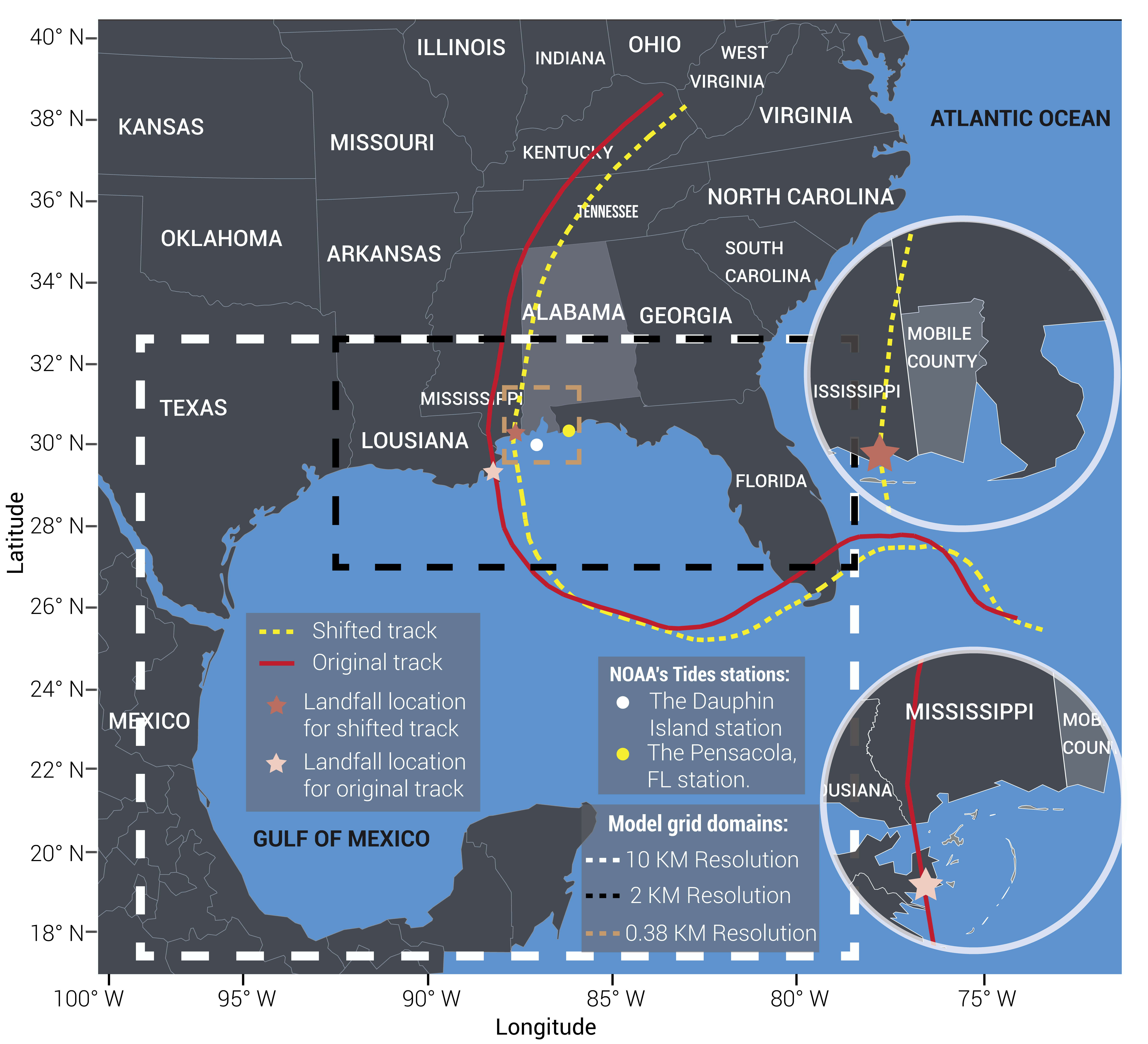
Hydrologic and hydrodynamic models were developed to model the hurricane hazard. The hydrologic analysis was conducted on Delft3d. To simulate the hurricane wind profile throughout its track, the analysis domain must include the point of hurricane formation to capture the water propagated from the Gulf of Mexico (GOM) accurately. Accordingly, a nesting grid modeling technique is used to simulate a broad selection of spatial scales. A large lower resolution grid of about 10 km is chosen to cover the GOM region as the first stage of the analysis. Then, the output information from the GOM model is passed to a higher resolution grid of about 2 km that covers the northern part of the Gulf (NG). Finally, the results of the previous two domains are passed to the highest resolution grid domain of about 0.38 km surrounding Mobile Bay (MB). Bathymetry and topography data are based on the U.S. Coastal Relief Model (CRM) which has a horizontal resolution of three arc seconds (approximately 90 m). The vertical datum in the CRM model is mean sea level. In areas where the CRM data are not available, the General Bathymetric Chart of the Oceans (900 m horizontal resolution) is used. The seafloor roughness factor is defined by the spatial variations of the Manning coefficient, which is extracted from the land use data using the National Land Cover Database (NLCD) and then transformed to compatible Manning’s values. (Adhikari et al., 2021)

Modeling domains, hurricane Katrina’s original, shifted track, and their landfall locations (Figure source: Abdelhafez et al., 2021)

2.2 Validation of the hazard modeling

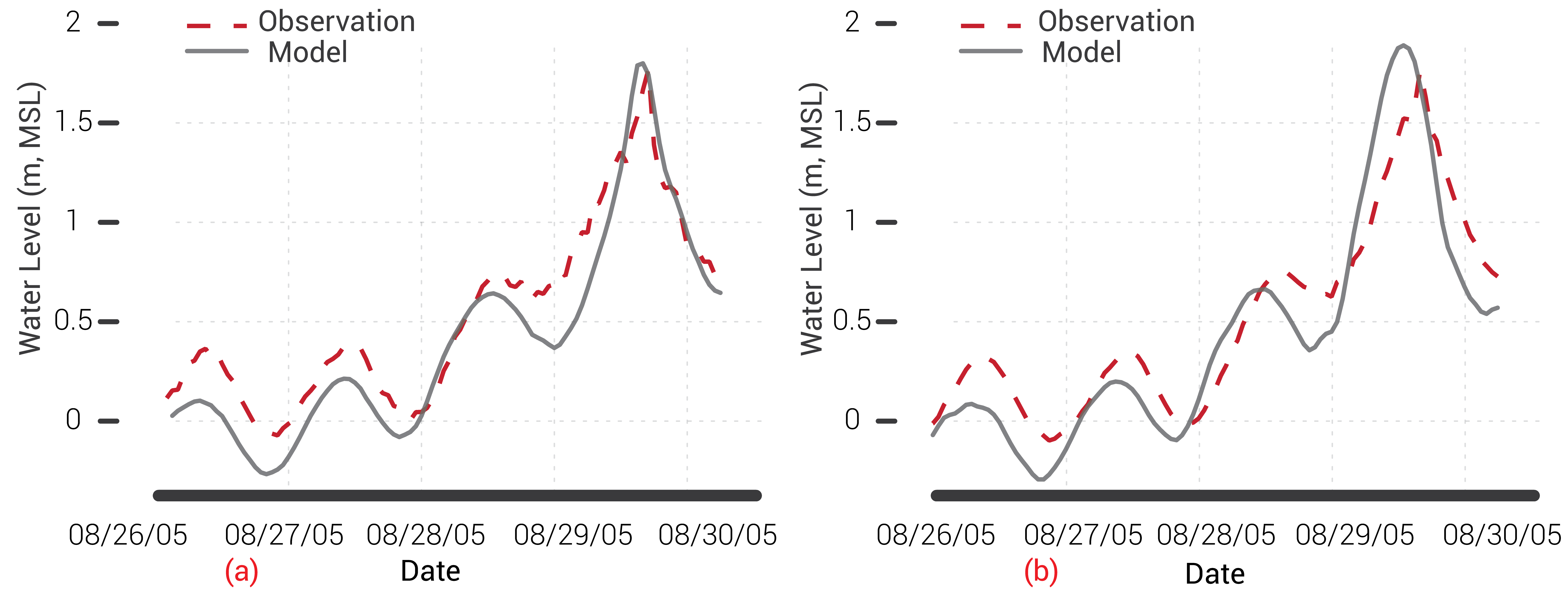
The accuracy of the storm surge model from Delft3D was tested using data obtained during Hurricane Katrina from the NOAA Tides and Currents stations at Dauphin Island, AL and at Pensacola, FL, as they were the only two stations that had recorded data during the hurricane. The simulation also captures the peak storm surge of about 3.5m in downtown Mobile, which matches the FEMA high water marks at this location More details about the validation can be found in Adhikari et al. (2021).

(a) Dauphin island and (b) Pensacola, FL observation stations. (Figure source: Adhikari et al., 2021)

2.3 Storm surge coupled with the projected sea level rise

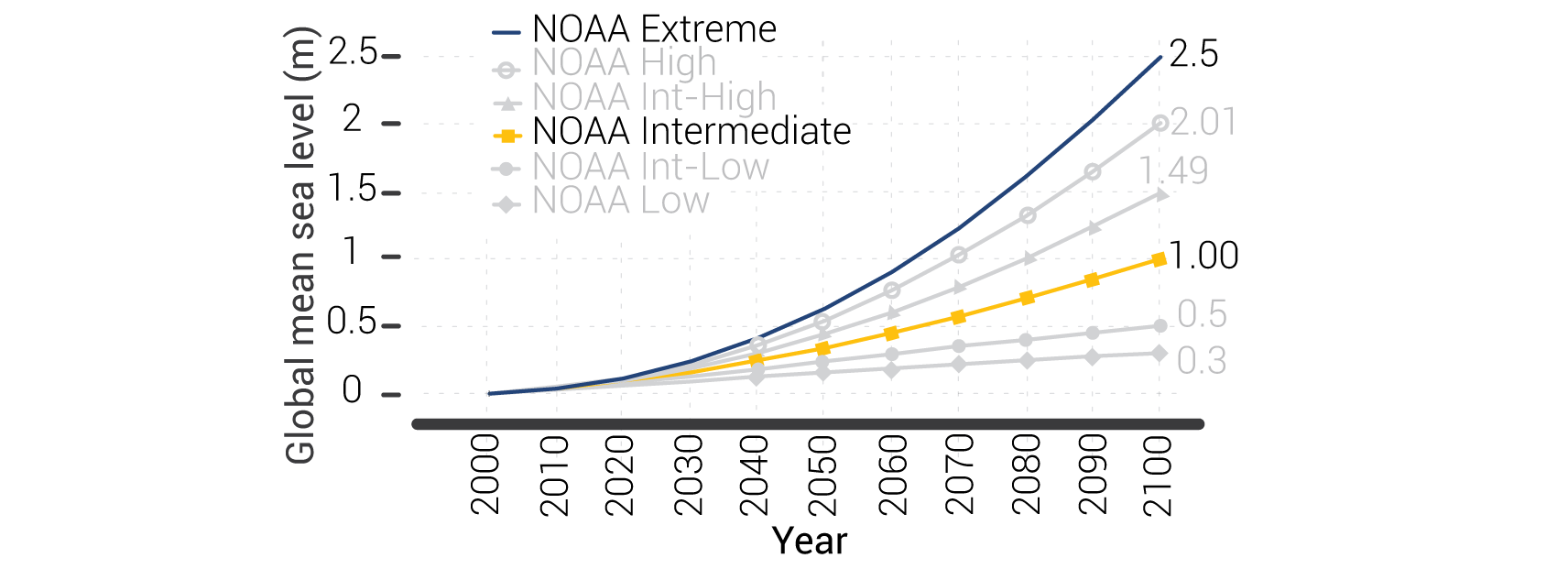
The actual hydrodynamic parameters of water level and characteristics of the existing hurricane track are used in the baseline storm surge scenario, illustrated in the previous Figure, while for the future scenarios, the water level and characteristics were updated by the Army Corps of Engineers for Dauphin Island gauge station based on NOAA climate projections scenarios. Two sea level rise scenarios are selected to represent the intermediate and extreme scenarios in NOAA’s scale. (Adhikari et al., 2021)

NOAA's global mean sea level rise projection (Figure source: Abdelhafez et al., 2021)

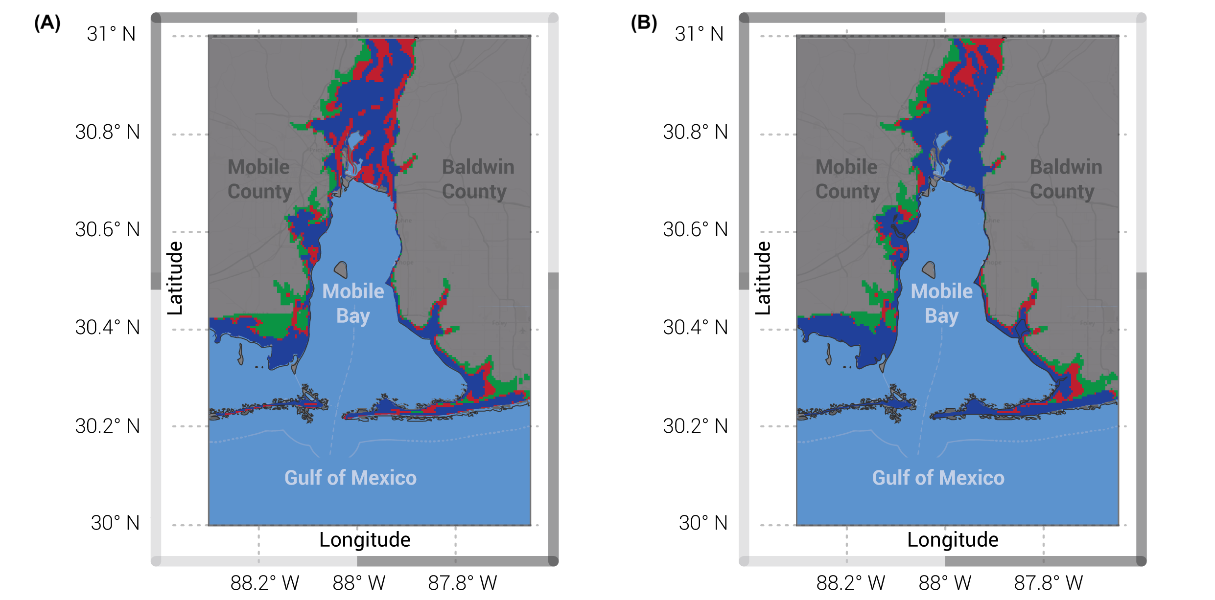
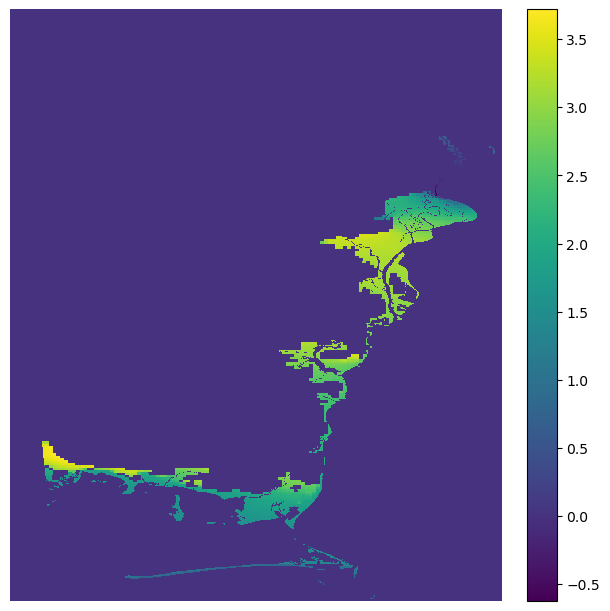
A raster map of the developed storm surge hazard coupled with projected SLR are shown in the figure below. The hazard data are available in terms of scenario-based with the following IDs in IN-CORE:

• Water level for natural hurricane Katrina in 2005 ID: 6420c6e6d9ae37665ff0d5f2

• Water level for natural hurricane Katrina coupled with NOAA intermediate SLR ID: 64222491d9ae37665ff0d5f3

• Water level for natural hurricane Katrina coupled with NOAA extreme SLR ID: 6422253cd9ae37665ff0d5f4

• Water level for shifted hurricane Katrina ID: 642d387bfde0f316c3493530

• Water level for shifted hurricane Katrina coupled with NOAA intermediate SLR ID: 642d38f1fde0f316c3493531

• Water level for shifted hurricane Katrina coupled with NOAA extreme SLR ID: 642d3c7763601e1e19241468

Inundations for (A) natural Hurricane Katrina track and (B) shifted Hurricane Katrina track. Blue color dominates the area inundated by the hurricane, red represents the extra area flooded by the hurricane coupled with NOAA intermediate SLR, and the green shows the inundated area by the hurricane coupled with NOAA extreme SLR (Figure source: Adhikari et al., 2021)

The following code reads the storm surge hazard data

# Surge Inundation Hazard Map based on the Hurricane Katrina in 2005 from IN-CORE
hazard_type = "Hurricane Surge"
Hurricane_Inundation_level_m_id = "6420c6e534810d74880b511e"   # Raster Map for the water levels in m

#visualize the surge Inundation hazard data 
Hurricane_water_m_dataset = Dataset.from_data_service(Hurricane_Inundation_level_m_id, DataService(client))
map1=viz.map_raster_overlay_from_file(Hurricane_water_m_dataset.get_file_path('tif'))
map1

/home/cnavarro/miniconda3/envs/pyincore-1.20.0/lib/python3.9/site-packages/osgeo/gdal.py:311: FutureWarning: Neither gdal.UseExceptions() nor gdal.DontUseExceptions() has been explicitly called. In GDAL 4.0, exceptions will be enabled by default.
  warnings.warn(

# add opacity control - NOTE: It takes time before the opacity takes effect.
map1.layers[1].interact(opacity=(0.0,1.0,0.01))

dataset = Dataset.from_data_service(Hurricane_Inundation_level_m_id, DataService(client))
map = viz.plot_raster_file_with_legend(dataset.get_file_path('tif'))
map

Dataset already exists locally. Reading from local cached zip.
Unzipped folder found in the local cache. Reading from it...

2.4 Exposure Modeling

Residential buildings dataset

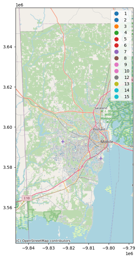
Data related to the building inventory in Mobile County, AL, were constructred by integrating the Microsoft Footprint (Bing Maps dataset), ATTOM (a real estate information database), and The National Structure Inventory (NSI). More information about the integration between the Microsoft Footprint and ATTOM datasets can be found in Abdelhafez et al., 2022. NSI was the main contributor to the residential buildings dataset, while ATTOM data were used when NSI data were missing.

# Mobile Residential Building Inventory from IN-CORE
Building_Inventory_id = "649361d8e435fd233fbbd1b3"

# visualize the building inventory
Mobile_Building_Inventory = Dataset.from_data_service(Building_Inventory_id, DataService(client))
map=viz.plot_map(Mobile_Building_Inventory, column="archetype", category=True, basemap=True)
map

# load building inventory as Geodataframe
filename = Mobile_Building_Inventory.get_file_path('shp')
print("The IN-CORE Dataservice has saved the Building Inventory on your local machine: "+filename)
bldg_inv_gdf = gpd.read_file(filename)
bldg_inv_gdf.head()

The IN-CORE Dataservice has saved the Building Inventory on your local machine: /home/cnavarro/.incore/cache_data/648c22dd689743dc9dedf242006adc5a9c21de9a89c016323dccfedef94f7737/649361d8e435fd233fbbd1b3/Mobile_Buildings_final_v2/Mobile_Buildings_final_v2.shp

	strctid	nsi_id	parid	struct_typ	year_built	no_stories	a_stories	b_stories	bsmt_type	sq_foot	...	ffe_elev	g_elev	archetype	arch_wind	arch_flood	arch_sw	csv_guid	csv_sector	csv_val_st	geometry
0	None	500671344	0	M	1965	1	0	0	S	1314.81	...	9.747187	9.594787	6	0	6	0	0	0	0	POLYGON ((-88.11035 30.69477, -88.11047 30.694...
1	None	501214248	0	M	1971	3	0	0	S	1000.00	...	6.791795	6.639395	8	0	8	0	0	0	0	POLYGON ((-88.08226 30.62174, -88.08246 30.621...
2	None	501088504	0	C	1982	1	0	0	S	3081.68	...	2.777907	2.625507	9	0	9	0	0	0	0	POLYGON ((-88.24389 30.39093, -88.24398 30.390...
3	None	500859644	0	M	1977	1	0	0	S	13000.00	...	62.463843	62.311443	15	0	15	0	0	0	0	POLYGON ((-88.14662 30.69472, -88.14678 30.694...
4	None	500768467	0	W	1947	1	0	0	S	33000.00	...	6.684362	6.531962	8	0	8	0	0	0	0	POLYGON ((-88.08436 30.68948, -88.08451 30.689...

5 rows × 39 columns

# Classification of the 165810 residential buildings in Mobile County 

bldg_inv_gdf.groupby(["arch_flood"], as_index=False)["guid"].count()

	arch_flood	guid
0	1	121621
1	2	8918
2	3	27848
3	4	3403
4	5	6949
5	6	2047
6	7	22
7	8	1047
8	9	2579
9	10	186
10	12	613
11	13	713
12	14	200
13	15	3827

# Galveston Hurricane flood fragility mappings for buildings
mapping_id = "62fefd688a30d30dac57bbd7"
fragility_service = FragilityService(client)
mapping_set = MappingSet(fragility_service.get_mapping(mapping_id))

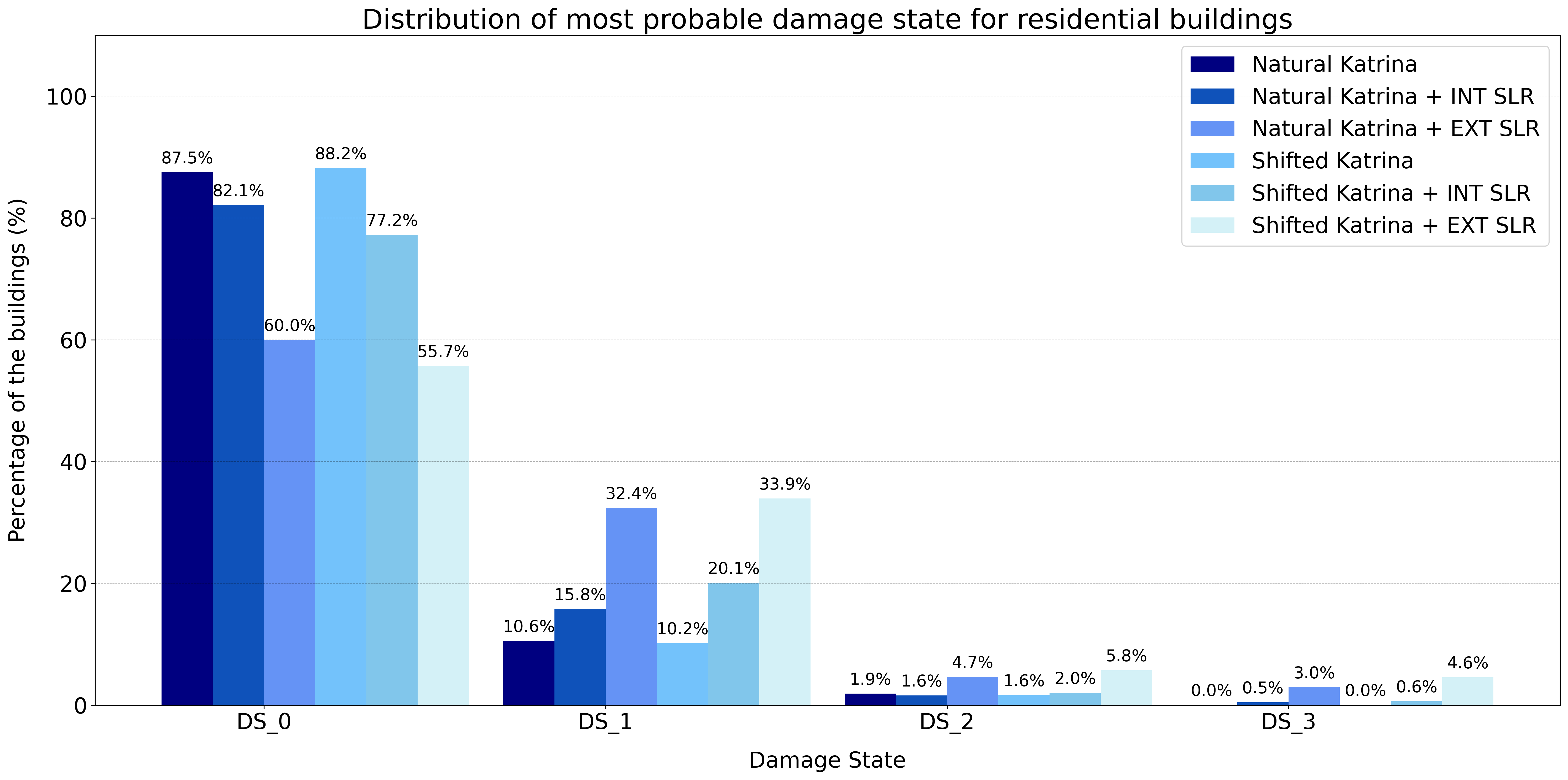
2.5 Building Damage Analysis

# Reading the Hazard type and the Hazard ID for the six hurricane and SLR scenarios
hazard_type = "hurricane" 

hurricane_hazard_dict = {}
hurricane_hazard_dict[0] = {'id': "6420c6e6d9ae37665ff0d5f2", 'name':'Natural Katrina'} 
hurricane_hazard_dict[1] = {'id': "64222491d9ae37665ff0d5f3", 'name':'Natural Katrina + INT SLR'}
hurricane_hazard_dict[2] = {'id': "6422253cd9ae37665ff0d5f4", 'name':'Natural Katrina + EXT SLR'}
hurricane_hazard_dict[3] = {'id': "642d387bfde0f316c3493530", 'name':'Shifted Katrina'}
hurricane_hazard_dict[4] = {'id': "642d38f1fde0f316c3493531", 'name':'Shifted Katrina + INT SLR'}
hurricane_hazard_dict[5] = {'id': "642d3c7763601e1e19241468", 'name':'Shifted Katrina + EXT SLR'}

bldg_dmg = BuildingStructuralDamage(client)

bldg_dmg.load_remote_input_dataset("buildings", Building_Inventory_id)
bldg_dmg.set_input_dataset("dfr3_mapping_set", mapping_set)

Dataset already exists locally. Reading from local cached zip.
Unzipped folder found in the local cache. Reading from it...

True

# Run the building damage analysis for the six hurricane and SLR scenarios

output_result=[]
output=[]
for i in range(0,len(hurricane_hazard_dict)): 
    result = []
    result2 = []
    result_name = "Mobile_bldg_natural_hurricane_dmg_result{0}".format(i)

    bldg_dmg.set_parameter("fragility_key", "Non-Retrofit Fragility ID Code")
    bldg_dmg.set_parameter("result_name", result_name)
    bldg_dmg.set_parameter("hazard_type", hazard_type)
    bldg_dmg.set_parameter("hazard_id", hurricane_hazard_dict[i]['id'])
    bldg_dmg.set_parameter("num_cpu", 8)
    bldg_dmg.run_analysis()
    # Retrieve result dataset
    result = bldg_dmg.get_output_dataset('ds_result')
    # Convert dataset to Pandas DataFrame
    result2 = result.get_dataframe_from_csv(low_memory=False)
    output.append(result2)
    output_result.append(result)
building_dmg_result_MC = output_result
building_dmg_result = output

# Select only the buildings exposed to the hazard sceanrios
output3=[]
for j in range(0,len(building_dmg_result)):
    output2 = building_dmg_result[j][building_dmg_result[j]['haz_expose']=='yes']
    output3.append(output2)
bdmg_df_expose = output3
    
    
# Add 'DS_max' attribute to bdmg_df_expose that provide the max damage state for each Mobile residential building
for j in range(0,len(bdmg_df_expose)):
    bdmg_df_expose[j]['DS_max'] = bdmg_df_expose[j].loc[:,['DS_0', 'DS_1', 'DS_2', 'DS_3']].idxmax(axis = 1)

/tmp/ipykernel_29603/2362224933.py:11: SettingWithCopyWarning: 
A value is trying to be set on a copy of a slice from a DataFrame.
Try using .loc[row_indexer,col_indexer] = value instead

See the caveats in the documentation: https://pandas.pydata.org/pandas-docs/stable/user_guide/indexing.html#returning-a-view-versus-a-copy
  bdmg_df_expose[j]['DS_max'] = bdmg_df_expose[j].loc[:,['DS_0', 'DS_1', 'DS_2', 'DS_3']].idxmax(axis = 1)
/tmp/ipykernel_29603/2362224933.py:11: SettingWithCopyWarning: 
A value is trying to be set on a copy of a slice from a DataFrame.
Try using .loc[row_indexer,col_indexer] = value instead

See the caveats in the documentation: https://pandas.pydata.org/pandas-docs/stable/user_guide/indexing.html#returning-a-view-versus-a-copy
  bdmg_df_expose[j]['DS_max'] = bdmg_df_expose[j].loc[:,['DS_0', 'DS_1', 'DS_2', 'DS_3']].idxmax(axis = 1)
/tmp/ipykernel_29603/2362224933.py:11: SettingWithCopyWarning: 
A value is trying to be set on a copy of a slice from a DataFrame.
Try using .loc[row_indexer,col_indexer] = value instead

See the caveats in the documentation: https://pandas.pydata.org/pandas-docs/stable/user_guide/indexing.html#returning-a-view-versus-a-copy
  bdmg_df_expose[j]['DS_max'] = bdmg_df_expose[j].loc[:,['DS_0', 'DS_1', 'DS_2', 'DS_3']].idxmax(axis = 1)
/tmp/ipykernel_29603/2362224933.py:11: SettingWithCopyWarning: 
A value is trying to be set on a copy of a slice from a DataFrame.
Try using .loc[row_indexer,col_indexer] = value instead

See the caveats in the documentation: https://pandas.pydata.org/pandas-docs/stable/user_guide/indexing.html#returning-a-view-versus-a-copy
  bdmg_df_expose[j]['DS_max'] = bdmg_df_expose[j].loc[:,['DS_0', 'DS_1', 'DS_2', 'DS_3']].idxmax(axis = 1)
/tmp/ipykernel_29603/2362224933.py:11: SettingWithCopyWarning: 
A value is trying to be set on a copy of a slice from a DataFrame.
Try using .loc[row_indexer,col_indexer] = value instead

See the caveats in the documentation: https://pandas.pydata.org/pandas-docs/stable/user_guide/indexing.html#returning-a-view-versus-a-copy
  bdmg_df_expose[j]['DS_max'] = bdmg_df_expose[j].loc[:,['DS_0', 'DS_1', 'DS_2', 'DS_3']].idxmax(axis = 1)
/tmp/ipykernel_29603/2362224933.py:11: SettingWithCopyWarning: 
A value is trying to be set on a copy of a slice from a DataFrame.
Try using .loc[row_indexer,col_indexer] = value instead

See the caveats in the documentation: https://pandas.pydata.org/pandas-docs/stable/user_guide/indexing.html#returning-a-view-versus-a-copy
  bdmg_df_expose[j]['DS_max'] = bdmg_df_expose[j].loc[:,['DS_0', 'DS_1', 'DS_2', 'DS_3']].idxmax(axis = 1)

# bdmg_df_expose[2][bdmg_df_expose[2]['DS_1']>0.01]

# bdmg_df_expose[5][bdmg_df_expose[5]['guid']=='cf0baa3f-9331-479e-805d-24958dbaec0d']

output5=[]
output7=[]
for k in range(0,len(bdmg_df_expose)):
    output4 = bdmg_df_expose[k]['DS_max'].value_counts(normalize=True).mul(100).index.tolist()
    output6 = bdmg_df_expose[k]['DS_max'].value_counts(normalize=True).mul(100).tolist()
    output5.append(output4)
    output7.append(output6)
    indexes = output5
    values  = output7
    

# Set plot parameters
fig, ax = plt.subplots(figsize=(20, 10), dpi=300)
width = 0.15 # width of bar
x = np.arange(len(indexes[0]))
x_labels = ['DS_0', 'DS_1', 'DS_2', 'DS_3']


containers = ax.bar(x , values[0], width, color='#000080', label='Natural Katrina')
containers = ax.bar(x  + width, values[1], width, color='#0F52BA', label='Natural Katrina + INT SLR')
containers = ax.bar(x  + (2 * width), values[2], width, color='#6593F5', label='Natural Katrina + EXT SLR')
containers = ax.bar(x  + (3 * width), values[3], width, color='#73C2FB', label='Shifted Katrina')
containers = ax.bar(x  + (4 * width), values[4], width, color='#81C6EB', label='Shifted Katrina + INT SLR')
containers = ax.bar(x  + (5 * width), values[5], width, color='#D4F1F7', label='Shifted Katrina + EXT SLR')



for bars in ax.containers:
    ax.bar_label(bars, labels = [f'{x.get_height()/100:.1%}' for x in bars], padding=5, fontsize = 15)
    
    
ax.set_ylabel('Percentage of the buildings (%)', labelpad=15, fontsize = 20)
ax.set_ylim(0,110)
ax.set_xticks(x + width + width/2)
ax.set_xticklabels(x_labels, fontsize = 20)
ax.set_xlabel('Damage State', labelpad=15, fontsize = 20)
ax.set_title('Distribution of most probable damage state for residential buildings',fontsize = 25)
ax.legend(fontsize = 20)
# ax('ytick', labelsize=10)    # fontsize of the tick labels
plt.tick_params(labelsize=20)
plt.grid(True, 'major', 'y', ls='--', lw=.5, c='k', alpha=.3)

fig.tight_layout()
plt.show()

# To visualize the output of Natural Katrina

bldg_results = pd.merge(bldg_inv_gdf, building_dmg_result[2], how = 'right', left_on = ['guid'], right_on=['guid'])

# To show the probability of exceedance of DS_1 > 0

bldg_results_F1 = bldg_results[(bldg_results['archetype'] > 0) & (bldg_results['DS_1'] > 0) ]
bldg_results_F1.explore(column='DS_1',cmap='Reds', 
                        popup=['guid','g_elev','ffe_elev','LS_0','LS_1','LS_2','DS_1','DS_2'
                                ],
                        tooltip=['guid','g_elev','ffe_elev','LS_0','LS_1','LS_2','DS_1','DS_2'
                                ],
                        tiles='CartoDB positron',
                        style_kwds=dict(color="Red",weight=5, opacity=0.4))

Make this Notebook Trusted to load map: File -> Trust Notebook

3. Monte Carlo Simulation (MCS)

output_mc=[]
num_samples = 500

for j in range(0,len(building_dmg_result_MC)):

    mc_bldg = MonteCarloLimitStateProbability(client)

    mc_bldg.set_input_dataset("damage", building_dmg_result_MC[j])  #  Load the Mobile building damage results dataset 
                                                             # generated from the previous model as an input
    mc_bldg.set_parameter("num_cpu", 8)
    mc_bldg.set_parameter("num_samples", num_samples)
    mc_bldg.set_parameter("damage_interval_keys", ["DS_0", "DS_1", "DS_2", "DS_3"])
    mc_bldg.set_parameter("failure_state_keys", ["DS_1", "DS_2", "DS_3"])

    mc_bldg.set_parameter("result_name", "storm_surge_mc_failure_probability_buildings") # name of csv file with results
    mc_bldg.run_analysis()  # Run the Monte Carlo Simulation module to obtain the building failure probabilities. 
    building_failure_probability = mc_bldg.get_output_dataset('failure_probability')  # get buildings failure probabilities
    result_mc = building_failure_probability.get_dataframe_from_csv()
    output_mc.append(result_mc)
df_bldg_fail = output_mc

df_bldg_fail[0][df_bldg_fail[0]['failure_probability']>0]

	guid	failure_probability
14	cf0baa3f-9331-479e-805d-24958dbaec0d	0.996
20	8b41d0c2-c9d4-4edc-b5b6-84cc0d49fd1e	0.288
40	586d5bf9-d0b6-4381-8de0-36865b1c8785	0.166
50	a6b1b40e-3a1b-477c-8b13-6a6bf757ffbb	0.262
55	a3eccde4-6b20-4f23-a48f-bb5a6364a458	0.082
...	...	...
179183	f688fb34-1986-49ca-93bf-3dbc5f80d701	0.918
179690	f8ed44ce-4267-4c69-a568-5051fca56479	0.006
179771	d51514c2-c273-49cd-bb03-f27f5edd43bc	0.054
179853	c19855bb-c248-4211-80f5-fd82bb73e2dc	0.270
179930	2ce2c3dd-2b9b-4568-a08f-b3f5b88be4e6	0.002

1834 rows × 2 columns

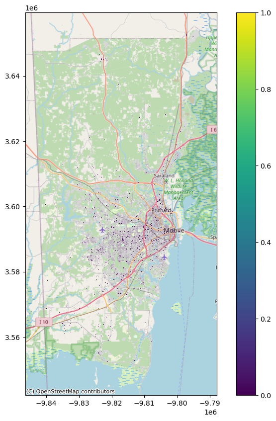
# To show the failure_probability Due to Katina scenario 
bldg_func_gdf = bldg_inv_gdf.merge(df_bldg_fail[0], on='guid')
viz.plot_gdf_map(bldg_func_gdf, column='failure_probability')

df_bldg_fail_1 = df_bldg_fail[0][['guid','failure_probability']]
df_bldg_fail_2 = df_bldg_fail[1][['failure_probability']]
df_bldg_fail_3 = df_bldg_fail[2][['failure_probability']]
df_bldg_fail_4 = df_bldg_fail[3][['failure_probability']]
df_bldg_fail_5 = df_bldg_fail[4][['failure_probability']]
df_bldg_fail_6 = df_bldg_fail[5][['failure_probability']]

df_bldg_fail_1.rename(columns = {'failure_probability':'fp_1'}, inplace = True) #Natural Katrina
df_bldg_fail_2.rename(columns = {'failure_probability':'fp_2'}, inplace = True) #Natural Katrina + INT SLR
df_bldg_fail_3.rename(columns = {'failure_probability':'fp_3'}, inplace = True) #Natural Katrina + EXT SLR
df_bldg_fail_4.rename(columns = {'failure_probability':'fp_4'}, inplace = True) #Shifted Katrina
df_bldg_fail_5.rename(columns = {'failure_probability':'fp_5'}, inplace = True) #Shifted Katrina + INT SLR
df_bldg_fail_6.rename(columns = {'failure_probability':'fp_6'}, inplace = True) #Shifted Katrina + EXT SLR
bldg_inv_gdf_all = pd.concat((df_bldg_fail_1,df_bldg_fail_2,df_bldg_fail_3,df_bldg_fail_4,df_bldg_fail_5,df_bldg_fail_6), axis=1)


bldg_inv_gdf_final = bldg_inv_gdf.merge(bldg_inv_gdf_all, on='guid')

/tmp/ipykernel_29603/678958795.py:9: SettingWithCopyWarning: 
A value is trying to be set on a copy of a slice from a DataFrame

See the caveats in the documentation: https://pandas.pydata.org/pandas-docs/stable/user_guide/indexing.html#returning-a-view-versus-a-copy
  df_bldg_fail_2.rename(columns = {'failure_probability':'fp_2'}, inplace = True) #Natural Katrina + INT SLR
/tmp/ipykernel_29603/678958795.py:10: SettingWithCopyWarning: 
A value is trying to be set on a copy of a slice from a DataFrame

See the caveats in the documentation: https://pandas.pydata.org/pandas-docs/stable/user_guide/indexing.html#returning-a-view-versus-a-copy
  df_bldg_fail_3.rename(columns = {'failure_probability':'fp_3'}, inplace = True) #Natural Katrina + EXT SLR
/tmp/ipykernel_29603/678958795.py:11: SettingWithCopyWarning: 
A value is trying to be set on a copy of a slice from a DataFrame

See the caveats in the documentation: https://pandas.pydata.org/pandas-docs/stable/user_guide/indexing.html#returning-a-view-versus-a-copy
  df_bldg_fail_4.rename(columns = {'failure_probability':'fp_4'}, inplace = True) #Shifted Katrina
/tmp/ipykernel_29603/678958795.py:12: SettingWithCopyWarning: 
A value is trying to be set on a copy of a slice from a DataFrame

See the caveats in the documentation: https://pandas.pydata.org/pandas-docs/stable/user_guide/indexing.html#returning-a-view-versus-a-copy
  df_bldg_fail_5.rename(columns = {'failure_probability':'fp_5'}, inplace = True) #Shifted Katrina + INT SLR
/tmp/ipykernel_29603/678958795.py:13: SettingWithCopyWarning: 
A value is trying to be set on a copy of a slice from a DataFrame

See the caveats in the documentation: https://pandas.pydata.org/pandas-docs/stable/user_guide/indexing.html#returning-a-view-versus-a-copy
  df_bldg_fail_6.rename(columns = {'failure_probability':'fp_6'}, inplace = True) #Shifted Katrina + EXT SLR

bldg_inv_gdf_nan = bldg_inv_gdf_final
bldg_inv_gdf_nan.replace(0, np.nan, inplace=True)

#To get number of Builidngs with failure_probability >0 for fp_1 to fp_6
bldg_inv_gdf_group = bldg_inv_gdf_nan.groupby(["archetype"], as_index=False).count()
bldg_inv_gdf_group = bldg_inv_gdf_group[['archetype','nsi_id','fp_1','fp_2','fp_3','fp_4','fp_5','fp_6']]
bldg_inv_gdf_group

	archetype	nsi_id	fp_1	fp_2	fp_3	fp_4	fp_5	fp_6
0	1	121621	857	4635	8926	1491	5458	9890
1	2	8918	49	333	721	84	434	772
2	3	27848	312	1300	2819	461	1610	3105
3	4	3403	9	104	238	33	130	295
4	5	6949	162	449	760	273	507	802
5	6	2047	16	85	182	33	111	200
6	7	22	1	2	5	1	3	5
7	8	1047	32	84	142	47	94	151
8	9	2579	268	492	648	341	535	682
9	10	186	0	5	12	0	7	13
10	12	613	5	22	41	12	23	47
11	13	713	11	45	87	21	60	91
12	14	200	11	30	47	18	36	55
13	15	3827	101	270	486	168	319	524